Usage
Olfactory Transduction Library
In this notebook, we demonstrate the various ways that the Olftrans
package is to be consumed by end-users.
import os
import matplotlib.pyplot as plt
import numpy as np
1. Estimating Binding & Dissociation Rates from Data
In this section, we show an example of estimating binding and dissociation rates from spike rate data. The data that we will use is from Hallem & Carlson 2006. The data shows the steady-state spike rates of odorant-receptor pairs under a step concentration input of 100 ppm.
The processed data is available in the Olftrans package as
olftrans.data.HallemCarlson.DATA.
Assumptions and Data Pre-processing
Steady-State Response Assumption:
Note that from the original 2006 publication’s Experimental Procedure Section: > Responses were quantified by subtracting the number of impulses in 500 ms of unstimulated activity from the number of impulses in the 500 ms following odorant stimulation, unless otherwise indicated.
We assume that 500 ms is sufficient for the response to reach steady-state.
Response level calculation:
Note that from the original 2006 publication’s Figure 1 Caption: > Responses of each receptor to the diluent were subtracted from each odorant response
To take into account the spontaneous firing rate of OSNs expressing each receptor type, we add the spontaneous firing rate to the reported spike rate by Hallem & Carlson. Note that this is consistent with the procedure in Stevens 2016 PNAS
Negative Spike Rate:
Even after adding the spontaneous firing rates, some of the firing rates are still negative. As such, we recify the resulting spike rate to be non-negative. Note that this is consistent with the procedure in Stevens 2016 PNAS
from olftrans import olftrans
from olftrans import data
data.HallemCarlson.DATA
2a |
7a |
9a |
10a |
19a |
22a |
23a |
33b |
35a |
43a |
43b |
47a |
47b |
49b |
59b |
65a |
67a |
67c |
82a |
85a |
85b |
85f |
88a |
98a |
|
|---|---|---|---|---|---|---|---|---|---|---|---|---|---|---|---|---|---|---|---|---|---|---|---|---|
ammonium hydroxide |
11 |
0 |
35 |
24 |
30 |
17 |
7 |
16 |
21 |
20 |
5 |
17 |
39 |
12 |
7 |
21 |
27 |
16 |
18 |
8 |
28 |
24 |
26 |
36 |
putrescine |
14 |
0 |
29 |
0 |
20 |
16 |
7 |
21 |
17 |
4 |
3 |
0 |
22 |
1 |
4 |
16 |
7 |
12 |
12 |
1 |
37 |
15 |
20 |
29 |
cadaverine |
9 |
0 |
24 |
0 |
24 |
17 |
2 |
18 |
29 |
11 |
14 |
0 |
31 |
6 |
9 |
17 |
3 |
20 |
14 |
3 |
42 |
23 |
26 |
33 |
g-butyrolactone |
17 |
51 |
56 |
8 |
22 |
47 |
13 |
32 |
98 |
9 |
21 |
7 |
56 |
7 |
18 |
24 |
136 |
26 |
9 |
6 |
60 |
30 |
28 |
41 |
g-hexalactone |
23 |
0 |
121 |
32 |
27 |
144 |
21 |
50 |
188 |
29 |
32 |
25 |
11 |
7 |
20 |
36 |
58 |
46 |
21 |
11 |
66 |
61 |
29 |
36 |
We can then calculate the affinity values of the odorant-receptor pairs based on the data.
spike_rates = data.HallemCarlson.DATA[~data.HallemCarlson.DATA.isna()].values
hallem_carlson_est = olftrans.estimate(amplitude=100., resting_spike_rate=8., steady_state_spike_rate=spike_rates, decay_time=0.1)
The estimation result hallem_carlson_est is a dataclass that
contains estimated affinity values in hallem_carlson_est.affs
attribute. We can save the estimated affinity values into another
dataframe as follows.
hallem_carlson_affs = data.HallemCarlson.DATA.copy()
hallem_carlson_affs[~hallem_carlson_affs.isna()] = hallem_carlson_est.affs
hallem_carlson_affs
2a |
7a |
9a |
10a |
19a |
22a |
23a |
33b |
35a |
43a |
43b |
47a |
47b |
49b |
59b |
65a |
67a |
67c |
82a |
85a |
85b |
85f |
88a |
98a |
|
|---|---|---|---|---|---|---|---|---|---|---|---|---|---|---|---|---|---|---|---|---|---|---|---|---|
ammonium hydroxide |
0.000115672 |
1e-08 |
0.00209477 |
0.000976631 |
0.00150285 |
0.000521254 |
1e-08 |
0.000443275 |
0.000801621 |
0.000746741 |
1e-08 |
0.000521254 |
0.0025163 |
0.000176793 |
1e-08 |
0.000801621 |
0.00120942 |
0.000443275 |
0.000603536 |
1e-08 |
0.00130248 |
0.000976631 |
0.0011201 |
0.00219478 |
putrescine |
0.000301777 |
1e-08 |
0.00139946 |
1e-08 |
0.000746741 |
0.000443275 |
1e-08 |
0.000801621 |
0.000521254 |
1e-08 |
1e-08 |
1e-08 |
0.000858196 |
1e-08 |
1e-08 |
0.000443275 |
1e-08 |
0.000176793 |
0.000176793 |
1e-08 |
0.00229827 |
0.000370178 |
0.000746741 |
0.00139946 |
cadaverine |
1.07163e-05 |
1e-08 |
0.000976631 |
1e-08 |
0.000976631 |
0.000521254 |
1e-08 |
0.000603536 |
0.00139946 |
0.000115672 |
0.000301777 |
1e-08 |
0.00161874 |
1e-08 |
1.07163e-05 |
0.000521254 |
1e-08 |
0.000746741 |
0.000301777 |
1e-08 |
0.00288659 |
0.000916515 |
0.0011201 |
0.00186734 |
g-butyrolactone |
0.000521254 |
0.00447951 |
0.00577908 |
1e-08 |
0.000858196 |
0.00365108 |
0.000237298 |
0.00174012 |
10 |
1.07163e-05 |
0.000801621 |
1e-08 |
0.00577908 |
1e-08 |
0.000603536 |
0.000976631 |
10 |
0.0011201 |
1.07163e-05 |
1e-08 |
0.00675985 |
0.00150285 |
0.00130248 |
0.00275671 |
g-hexalactone |
0.000916515 |
1e-08 |
10 |
0.00174012 |
0.00120942 |
10 |
0.000801621 |
0.00425483 |
10 |
0.00139946 |
0.00174012 |
0.0010386 |
0.000115672 |
1e-08 |
0.000746741 |
0.00219478 |
0.00624765 |
0.00346843 |
0.000801621 |
0.000115672 |
0.00925384 |
0.00703414 |
0.00139946 |
0.00219478 |
Note that since peak response was not reported in Hallem&Carlson 2006, we cannot estimate dissociation rate directly. However, the dissociation rate is the reciprocal of the decay time for the OSN activity to settle from steady-state response to resting response after odorant offset.
Assuming that the decay_time is 100 ms, the dissociation rate should
be \(10 s^{-1}\), which is the value given in
hallem_carlson_est.dr.
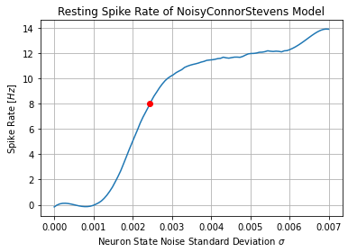
2. Computing Resting Spike Rate of BSG
OSNs are spontaneously firing neurons whose spiking mechanism is modeled
by a ConnorStevens neuron model with noisy state values. The state
parameters are perturbed by a brownian motion whose standard deviation
value sigma controls the resting spike rate of the neuron.
Given the Connor-Stevens neuron model, we can fix all other parameters
except for sigma and vary sigma to obtain the resting spike
rate. This sigma-spike rate relationship can then be used to
estimate the sigma parameter given resting spike rates.
from olftrans.neurodriver import model as nd

dt = 1e-5
repeat = 50
sigmas = np.linspace(0,0.007,100)
_, rest_fs = nd.compute_resting(
    nd.NoisyConnorStevens, 'sigma', sigmas/np.sqrt(dt), dt=dt, dur=2.,
    repeat=repeat, save=True, smoothen=True, savgol_window=31, savgol_order=4
)
Resting Spike Rate NoisyConnorStevens - Against sigma: 100%|██████████| 200000/200000 [00:26<00:00, 7635.25it/s]
target_resting_rate = 8. # Hz
target_sigma = np.interp(target_resting_rate, xp=rest_fs, fp=sigmas)
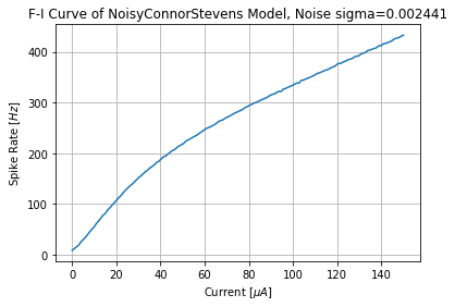
3. Computing BSG F-I Curve
Once a sigma value is found for a BSG neuron, we can then find the
Frequency-Current curve of a given neuron model. Obtaining the F-I curve
will help us estimate the OTP output current from the OSN’s output spike
rate.
from olftrans import data
from olftrans.neurodriver import model as nd

dt = 1e-5
repeat = 50
Is = np.linspace(0,150,150)
sigma = 0.0024413599558694506
_, fs = nd.compute_fi(
    nd.NoisyConnorStevens, Is, dt=dt, dur=3.,
    repeat=repeat, save=True,
    neuron_params={'sigma':sigma/np.sqrt(dt)}
)
F-I NoisyConnorStevens: 100%|██████████| 300000/300000 [00:44<00:00, 6670.95it/s]
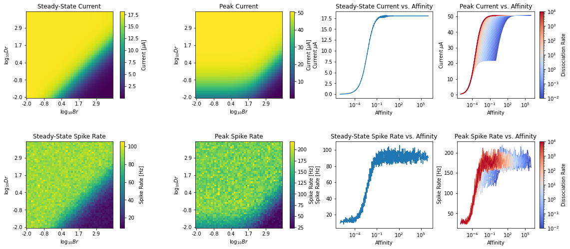
4. Computing Peak and Steady State Response of OTP
Once the F-I curve is found, it can be used to estimate the output current of OTP model to give rise to the observed spike rate at the output of OSN Axon-Hillock.
import os
import matplotlib.pyplot as plt
import numpy as np
from olftrans.neurodriver import model as nd

dt = 1e-5
brs = 10**np.linspace(-2, 4, 100)
drs = 10**np.linspace(-2, 4, 100)
amplitude = 100.
_,_,I_ss,I_peak = nd.compute_peak_ss_I(brs, drs, dt=dt, dur=4., start=0.5, save=True, amplitude=amplitude)
OTP Currents: 100%|██████████| 400000/400000 [01:03<00:00, 6272.69it/s]
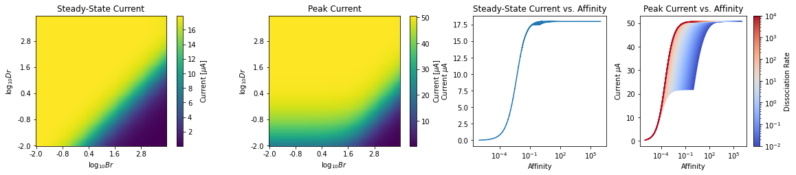
4.1 Infer Mapping from Affinity -> Steady-State Spike-Rate
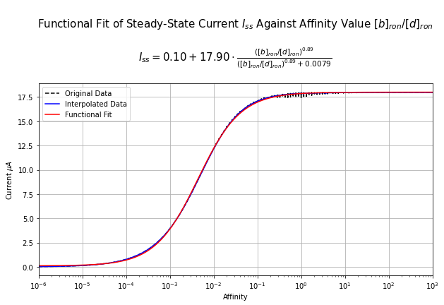
From steady-state spike rate, the affinity value can be estimated either by data interpolation or parametrically by first fitting a function to the spike-rate vs. affinity relationship.
Note that this can only be done robustly for the steady-state vs. affinity relationship (and not the other relationships above) because data reveals that such relationship strongly resembles a hill function.
As such, we use Differential Evolution to first estimate the parameter of a hill function that maps affinity value to steady-state output current of OTP and use the inverse of this function to estimate the affinity value from a given steady-state OTP current.
Note: Because the steady-state current of OTP model follows a hill function shape, it is nonnegative and saturates at a finite value. For steady-state currents outside of this range, the input affinity value cannote be estimated. As such, we clip the steady-state current value to be between the supported range beforing estimating its associated affinity value.
from scipy.optimize import differential_evolution
affs_intp = 10**np.linspace(-6,3,1000)
I_ss_flat = I_ss.ravel()
idx = np.argsort(affs)
ss_intp = np.interp(affs_intp, affs[idx], I_ss_flat[idx])
hill_f = lambda x, a,b,c,n: b + a*x**n/(x**n+c)
def cost(x, aff, ss):
    a,b,c,n = x
    pred = hill_f(aff,a,b,c,n)
    return np.linalg.norm(pred-ss)
bounds = [(0,100), (0, 100), (0,100), (.5, 2.)]
diffeq_ss = differential_evolution(cost, bounds, tol=1e-4, args=(affs_intp, ss_intp), disp=False)
def inverse_hill_f(y,a,b,c,n, x_ref):
    res = np.power(c*(y-b)/(a-(y-b)), 1./n)
    res[y<b] = x_ref.min()
    res[(y-b) > a] = x_ref.max()
    return res
5. Computing Peak and Steady State Response of OTP-BSG Cascade
Instead of going from Spike Rates -> Current -> Affinity, we can also go directly from Spike Rate -> Affininty. To do this, we will need to estimate the spike rate of the OTP-BSG cascade under step input waveform.
Note: because of the complexity of this estimation task, the code below takes significantly longer to run.
import os
import matplotlib.pyplot as plt
import numpy as np
from olftrans.neurodriver import model as nd

dt = 8e-6
brs = 10**np.linspace(-2, 4, 50)
drs = 10**np.linspace(-2, 4, 50)
repeat = 30
amplitude = 100.
_,_,I_ss,I_peak,f_ss,f_peak = nd.compute_peak_ss_spike_rate(brs, drs, dt=dt, dur=3., start=0.5, repeat=repeat, save=False, amplitude=amplitude)
Computing Peak and Steady State Currents
Computing Peak and Steady State Spike Rates
Computing PSTH...: 100%|██████████| 2500/2500 [15:53<00:00, 2.62it/s]
6. Working with Other FBL Packages
OlfTrans is intended to be used in conjuction with other FBL
packages. To make OlfTrans compatible with other executable
circuits, we define an olftrans.fbl module that exposes a class
olftrans.fbl.FBL that has the following attributes (among others,
see documentation for further details):
graph: anetworkx.MultiDiGraphinstance that defines the executable circuit comprised of OTP-BSG cascadesinputs: a dictionary of form{var: uids}that define the input variables and input nodes of the graphoutputs: a dictionary of form{var: uids}that define the output variables and output nodes of the graph
Additionally, we provide 2 pre-computed FBL instances using
Drosophila larva and adult data respectively:
olftrans.fbl.LARVA:FBLinstance using data from Kreher et al. 2005olftrans.fbl.Adult:FBLinstance using data from Hallem & Carlson. 2006
from olftrans import fbl
fbl.LARVA.config
Config(NR=21, NO=array([1, 1, 1, 1, 1, 1, 1, 1, 1, 1, 1, 1, 1, 1, 1, 1, 1, 1, 1, 1, 1]), affs=array([0., 0., 0., 0., 0., 0., 0., 0., 0., 0., 0., 0., 0., 0., 0., 0., 0.,
       0., 0., 0., 0.]), drs=array([10., 10., 10., 10., 10., 10., 10., 10., 10., 10., 10., 10., 10.,
       10., 10., 10., 10., 10., 10., 10., 10.]), receptor_names=['Or0', 'Or1', 'Or2', 'Or3', 'Or4', 'Or5', 'Or6', 'Or7', 'Or8', 'Or9', 'Or10', 'Or11', 'Or12', 'Or13', 'Or14', 'Or15', 'Or16', 'Or17', 'Or18', 'Or19', 'Or20'], resting=8.0, sigma=0.002442364106413095)
fbl.LARVA.graph
<networkx.classes.multidigraph.MultiDiGraph at 0x7f6241288828>
fbl.LARVA.affinities
30a |
42a |
45a |
45b |
49a |
69a |
67b |
74a |
85c |
94a |
94b |
|
|---|---|---|---|---|---|---|---|---|---|---|---|
ethyl acetate |
0.000702006 |
10 |
0.0062682 |
0.000902033 |
0.000902033 |
0.00555246 |
0.0020684 |
0.00303725 |
0.00598167 |
0.00120451 |
0.00131617 |
pentyl acetate |
0.000702006 |
0.0215691 |
10 |
0.00143349 |
0.00338442 |
0.00218748 |
10 |
0.00570972 |
10 |
0.00312099 |
0.00382387 |
ethyl butyrate |
0.000502663 |
10 |
0.00951996 |
0.000733843 |
0.00131617 |
0.00149608 |
0.000799287 |
0.0032945 |
0.0215691 |
0.00104804 |
0.00178211 |
methyl salicylate |
0.00218748 |
0.00521272 |
0.00097371 |
0.0001385 |
0.000248212 |
0.00120451 |
0.000368073 |
0.00149608 |
0.0027974 |
0.0020684 |
0.00312099 |
1-hexonol |
0.000902033 |
10 |
10 |
0.00257565 |
0.00406467 |
0.00120451 |
10 |
10 |
10 |
0.00474388 |
0.00320672 |
fbl.LARVA.inputs
{'conc': array(['OSN-OTP-Or0-O0', 'OSN-OTP-Or1-O0', 'OSN-OTP-Or2-O0',
        'OSN-OTP-Or3-O0', 'OSN-OTP-Or4-O0', 'OSN-OTP-Or5-O0',
        'OSN-OTP-Or6-O0', 'OSN-OTP-Or7-O0', 'OSN-OTP-Or8-O0',
        'OSN-OTP-Or9-O0', 'OSN-OTP-Or10-O0', 'OSN-OTP-Or11-O0',
        'OSN-OTP-Or12-O0', 'OSN-OTP-Or13-O0', 'OSN-OTP-Or14-O0',
        'OSN-OTP-Or15-O0', 'OSN-OTP-Or16-O0', 'OSN-OTP-Or17-O0',
        'OSN-OTP-Or18-O0', 'OSN-OTP-Or19-O0', 'OSN-OTP-Or20-O0'],
       dtype='<U15')}
fbl.LARVA.outputs
{'V': array(['OSN-BSG-Or0-O0', 'OSN-BSG-Or1-O0', 'OSN-BSG-Or2-O0',
        'OSN-BSG-Or3-O0', 'OSN-BSG-Or4-O0', 'OSN-BSG-Or5-O0',
        'OSN-BSG-Or6-O0', 'OSN-BSG-Or7-O0', 'OSN-BSG-Or8-O0',
        'OSN-BSG-Or9-O0', 'OSN-BSG-Or10-O0', 'OSN-BSG-Or11-O0',
        'OSN-BSG-Or12-O0', 'OSN-BSG-Or13-O0', 'OSN-BSG-Or14-O0',
        'OSN-BSG-Or15-O0', 'OSN-BSG-Or16-O0', 'OSN-BSG-Or17-O0',
        'OSN-BSG-Or18-O0', 'OSN-BSG-Or19-O0', 'OSN-BSG-Or20-O0'],
       dtype='<U15'),
 'spike_state': array(['OSN-BSG-Or0-O0', 'OSN-BSG-Or1-O0', 'OSN-BSG-Or2-O0',
        'OSN-BSG-Or3-O0', 'OSN-BSG-Or4-O0', 'OSN-BSG-Or5-O0',
        'OSN-BSG-Or6-O0', 'OSN-BSG-Or7-O0', 'OSN-BSG-Or8-O0',
        'OSN-BSG-Or9-O0', 'OSN-BSG-Or10-O0', 'OSN-BSG-Or11-O0',
        'OSN-BSG-Or12-O0', 'OSN-BSG-Or13-O0', 'OSN-BSG-Or14-O0',
        'OSN-BSG-Or15-O0', 'OSN-BSG-Or16-O0', 'OSN-BSG-Or17-O0',
        'OSN-BSG-Or18-O0', 'OSN-BSG-Or19-O0', 'OSN-BSG-Or20-O0'],
       dtype='<U15')}